Asterisms

When you look up at the night sky, the first thing that catches your attention is that you can trace imaginary lines joining the stars and you can create any shapes you want. It is very easy to imagine fantastic animals or all kinds of imaginary characters with a thousand and one shapes. Then, you just have to let your imagination fly and endow the imagined shape with a life, a past, and events that have caused it to end up in the sky represented by the chosen stars.

The marvellous part is that humanity has spent its entire existence doing precisely that. There has always been someone who has looked up at the sky and imagined a world full of creatures and beings that, whether for their goodness or wickedness, have ended up fixed among the stars. Culture and era do not matter. Everyone has an imaginary represented in the celestial vault and it is incredibly rich. For good reason. The human imagination has no limits and that is absolutely marvellous. In reality, the underlying idea of creating these imaginary stellar figures is to try to bring a little order and make it easier so that when someone talks about a part of the sky, others know which part they are referring to.

These celestial forms receive the generic name of asterism. This word comes from Ancient Greek (asterismwhat does literally mean “star cluster “stellar configuration”. Asterism derives from star (star), which means star. The term later passes into Latin as asterism and, from here, it enters modern languages (Catalan, Spanish, French, English...) keeping its original meaning almost intact.

It appears that the first graphic representation of an asterism would be in Lascaux Cave, France. Among thousands of paintings of various animals, painted about 16,500 years ago before the present, in the middle of the Mesolithic, there would be some black dots that could be the representation of the Pleiades and of the Hyades, both star clusters located in the constellation of Taurus. Not everyone agrees, however.

Instead, the first written reference would be much more modern and would be represented by what appears to be humanity's first astronomical treatise. This is composed of two clay tablets written in cuneiform of Babylonian origin and which would describe different aspects of the astronomy and astrology of this Mesopotamian culture. These tablets are known as MUL.APIN and, according to some recent astrometric work, would have an age of around 3,370 +/- 100 years before present. While it would seem that the name refers to the asterism of Cassiopeia, the treatise would describe 17 asterisms, among which would stand out Taurus, Perseus, Orion i Auriga, among others.

Most of the most identifiable asterisms in the northern hemisphere in Western culture reach us through Greco-Roman tradition, although many of them have much older roots, especially in the Mesopotamian cosmology of the 3rd–2nd millennium BC. Proof of this are the names of Orion, which in Mesopotamian culture is named SIPA.ZI.AN.NA and could be translated as Shepherd of Heaven, and which in Greek culture becomes the giant hunter we already know. In fact, Greek culture inherits this Mesopotamian cosmology and does three fundamental things:

1. Narrativize creating a whole myth-rich world around the most identifiable asterisms and anthropomorphizing them by assimilating them to gods that interact with human beings.
2. Fix names of many of the asterisms that we know and that, subsequently, Roman culture would pass into Latin and spread throughout the Roman Empire, creating a vast, highly homogeneous culture. Later, all these names pass into our language.
3. They are transmitting the system in medieval and modern Europe through a large number of writings that have come down to us, such as those of Homer, Hesiod, Aratus, and Ptolemy. These writings, continually copied for centuries in monasteries throughout Europe, would become the basis of later astronomical revolutions.

Over time, with technological and scientific progress, we now know that asterisms are nothing more than curiosities from the past that we use to amuse ourselves. The great advantage is the same as it was in the past: they allow us to orient ourselves in the sky and explain it to others when we do an outdoor astronomy session. Now we know that the stars that make up the asterisms are not all in the same horizontal plane but are each at a different distance from Earth. The part that has always interested me is knowing how far away these stars are.

The European Space Agency's Gaia project, with the launch in 2013 of satellite which bears the same name, made it possible to achieve something that until then was unthinkable: to measure astrometric data such as position, luminosity, distance, temperature, chemical composition, and movement of nearly 2 billion celestial objects located around us with unprecedented precision. This project, still ongoing even though the satellite ceased to be operational on January 15, 2025, made it possible to create a very detailed map of our galaxy, the Milky Way, in an effort to decipher its origin and future evolution. The data produced within this project have been progressively released to the entire scientific community and the general public. The first data release took place on September 14, 2016, under the name of Gaia Data Release (DR) 1. On April 25, 2018, Gaia DR2 was released, and on December 3, 2020, it was Gaia DR3. Gaia DR4 is expected around December 2026, and the final data release (Gaia DR5) is not expected before 2030.

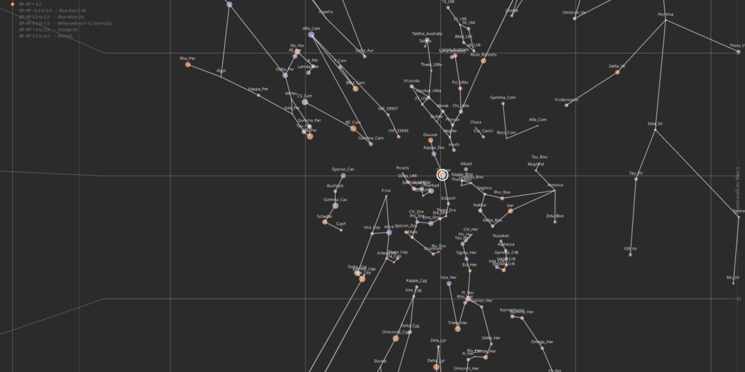
Since Gaia's astronomical data is publicly accessible, you only need a little programming to download it to your computer and explore the three-dimensional structure of the stars around us. Using the R programming language, which is free and available for multiple operating systems, I have developed a workflow to retrieve and analyze the astronomical data of over 200 stars and reconstruct in 3D the main asterisms of the northern hemisphere. The workflow uses three R scripts to identify the stars, retrieve their properties, and prepare the three-dimensional scene. Subsequently, a short Python script generates a standalone HTML file, whose interactive graphics are rendered by JavaScript inside a web browser.

The first R script identifies the stars that form each asterism. Although we know them by names like Deneb, Vega, or Arcturus, the objects in the Gaia catalog are identified by numerical codes. To find the correct correspondence, the script queries the SIMBAD astronomical database, which integrates stellar names, catalog identifiers, coordinates, and other published information. This identification stage is especially important in the case of double or multiple stars: a familiar name may refer to an entire stellar system rather than an individual component. For this reason, the script attempts to determine the exact identity of the star to be represented on the chart before retrieving its Gaia data.

The second R script retrieves the astrometric and photometric measurements available in Gaia Data Release 3, along with the distance estimates from the Bailer-Jones catalog. These data include stellar coordinates, proper motions, parallaxes, apparent magnitudes, colors and, when available, radial velocities. Distance is a particularly important and sometimes difficult quantity to estimate. Bailer-Jones's estimates combine Gaia observations with statistical information to infer stellar distances, including cases where the simple inversion of the measured parallax would be unreliable. However, there is no single method for determining distances suitable for all stars, especially in the case of very bright stars, multiple systems, or distant supergiants.

Not all stars have a useful Gaia measurement or a reliable Bailer-Jones distance. In these cases, the script can resort to a distance from another clearly identified catalog or derive an approximate distance from a sufficiently precise parallax. If the available measurements do not allow for a defensible distance to be obtained, the script logs this limitation rather than assigning the star the properties of a nearby but unrelated Gaia source. Some exceptional objects also require individually evaluated distance estimates from the scientific literature. The adopted distance, its uncertainty, and its source are preserved in the dataset so that the resulting three-dimensional reconstruction does not conceal these differences in reliability. When the necessary proper motion data are available, stellar positions are also referenced to a common epoch.

The third R script transforms the celestial coordinates and adopted distances into a three-dimensional Cartesian system. Right ascension and declination specify a direction on the celestial sphere, while the distance indicates how far along that direction the star is located. The combination of these three quantities makes it possible to place each star in physical space, with the three axes expressed in parsecs (1 pc ≈ 3.26 light-years). Unlike a previous version of these plots, which used a tangent plane projection for the two angular axes and parsecs only for the depth axis, the current reconstruction uses consistent physical units across all three dimensions. This allows one to explore the extent to which the familiar two-dimensional pattern of an asterism can differ from the actual spatial distribution of its stars.

The script also incorporates background stars from HYG star catalog, using their individual positions and distances instead of placing them on an artificial plane. Their colors are based on available photometric measurements, which provide an indication of stellar temperature: bluer stars tend to be hotter, while redder ones tend to be cooler. However, color is not a direct measurement of temperature, and some stars lack the photometric data necessary to assign them a reliable color. Legends relating to the size and color of the stars help interpret how these properties have been represented graphically.

Finally, the R script transfers the prepared scene to a rendering engine written in Python, which packages the astronomical data, controls, and graphics code into a single HTML file. The interactive visualization is generated by JavaScript using the browser's Canvas 2D graphics system, instead of the Plotly library for R used by my original version. As a result, each final chart can be opened directly in a web browser or embedded in a web page without visitors needing to install R, Python, or any other additional graphics software.

The chart initially opens in the mode Earth View, which shows the asterism as seen from our position in space. You can rotate and zoom this view, and then switch to the mode Explore 3D to move the camera through the same star model and discover the distances separating stars that apparently seem very close to each other in the night sky. Both visualizations are connected: Earth View it is simply a specific camera position within the 3D reconstruction and not an independent illustration. You can also adjust the size of the star markers, show the connections between the stars, and view their available properties by hovering the cursor over them.

An additional control allows compressing or exaggerating the represented depth. This can facilitate the exploration of asterisms with a very wide range of stellar distances, but it modifies their visual proportions, not the measured coordinates. The true-scale setting preserves the physical proportions of the reconstructed stellar positions and is the appropriate option when comparing their actual geometry.

Orion:

Cassiopeia

Cepheus

Minor spine:

Dragó:

Great Bear:

Hercules:

Crane:

Leo:

Taurus:

The ferryman:

Northern Crown:

Lira:

Edge

Exploring the cosmic web in three dimensions with public astronomical data

Since the data needed to reconstruct the large-scale structure of the nearby Universe is publicly available, all it takes is a bit of programming to download it, transform it into three-dimensional coordinates, and visualize it interactively. This is precisely what I have done in these three figures.

Although the three reconstructions may seem similar at first glance, they do not show the exact same thing. Two of them explore our relatively nearby cosmic neighborhood using the same galaxy catalog and the same density reconstruction, but at different scales and with different objectives. The third uses a completely different survey to look much further into the Universe.

From public catalogs to three-dimensional positions

I have used the free and cross-platform R programming language again to download and process the astronomical data.

For the two reconstructions of the nearby Universe I have used the 2MASS Redshift Survey (2MRS) public catalog, along with its subsequent redshift completeness table (redshift-completion table). The original catalog contains 44,599 galaxies and provides their position on the sky, infrared magnitude, and recession velocity.

A galaxy catalog typically provides two angular coordinates and a redshift (redshift), but not a calculated three-dimensional position. For this reason, the R script corrects the recession velocities to the Cosmic Microwave Background reference frame, converts the redshift into comoving distance, and transforms the resulting positions into supergalactic Cartesian coordinates. In this coordinate system, the supergalactic plane roughly follows the main distribution of nearby galaxies and galaxy clusters.

I combined the galaxy positions with the public density reconstruction Cosmicflows-4. Cosmicflows-4 is not just another galaxy catalog, but a three-dimensional density field reconstructed from galactic distances and peculiar velocities. Positive values represent regions with a matter density higher than the cosmic average, while negative values identify less dense regions.

For the deepest reconstruction I used the bright galaxy sample (Bright Galaxy Sample) de DESI Data Release 1. I had to convert the data for right ascension, declination, and redshift into equatorial Cartesian coordinates. Afterwards, I added the cosmic voids from the catalog DESIVAST, which identifies low-redshift cosmic voids using various numerical algorithms.

I performed the astronomical calculations and data preparation using R, and the calculated coordinates were compressed into compact 32-bit numeric buffers that were incorporated directly into the final HTML file.

Subsequently, JavaScript and the library Three.js They transfer these buffers to the graphics processor and render the galaxies as a reduced number of GPU objects. The Cosmicflows density surfaces are dynamically reconstructed in the browser using a type of algorithm. marching cubes.

Carrying out this division of tasks has been important because, while R has managed the scientific data, coordinate transformations, and selections, JavaScript has handled the interactive rendering.

---

1. The Local Void and neighboring structures

The first figure is an enlargement of the Universe within a radius of 500 million light-years from the Milky Way. It contains 32,838 galaxies from the 2MRS catalog and was conceived as a three-dimensional counterpart to the classical diagrams of the Buy Local and of the neighboring superclusters.

The concentric rings are separated by 100 million light-years and provide an immediate visual reference for scale. The names identify prominent voids, walls, galaxy clusters, and superclusters, while the vertical lines project these structures onto the supergalactic plane.

The red and magenta surfaces represent low-density regions reconstructed from Cosmicflows-4. The yellow surfaces indicate denser structures and can be toggled from the legend. The labeled positions should be interpreted as representative reference points: superclusters, walls, and voids are extensive structures that often have irregular boundaries or depend on the definition used.

This is the most suitable figure to identify the Local Void and understand its spatial relationship with the superclusters of Virgo, Hydra, Centaur, Perseus-Pisces i Coma.

---

2. The nearby large-scale cosmic web

The second reconstruction uses the same 2MRS and Cosmicflows-4 data sources, but expands the view to approximately 874 million light-years from the observer. It shows 43,461 galaxies.

All galaxies included in the Local Void atlas also appear in this more extensive reconstruction. Therefore, the atlas does not constitute an independent dataset, but rather a closer and much more annotated view of the central region of this map.

However, its objective is different. Instead of reproducing the appearance of a traditional astronomical atlas, this figure emphasizes the relationship between the observed distribution of galaxies and the reconstructed density field. The blue surfaces represent different levels of low density, while the orange surfaces indicate overdense regions. These surfaces make it possible to visualize how galaxy filaments and concentrations surround enormous, comparatively empty volumes.

This reconstruction is especially suited for exploring the general geometry of the nearby cosmic web and the spatial relationships between structures such as Laniakea, the Shapley Supercluster, the Perseus-Pisces Supercluster, the South Pole Wall and various large cosmic voids.

---

3. Looking much further with DESI

The third figure is fundamentally different. It uses 67,209 galaxies from the DESI bright galaxy sample and reaches much further into the Universe than the reconstructions based on 2MRS.

The color of the galaxies represents their redshift and, therefore, provides a rough indication of their distance and the time elapsed since their light was emitted. The transparent blue spheres represent the 80 largest inner voids identified by the algorithm VoidFinder within the DESIVAST catalog. Their dimensions are proportional to the effective radii of the catalog, which range approximately from 21.5 to 30.9 h⁻¹ megaparsecs.

These spheres should not be interpreted as perfectly spherical cosmic walls. Real cosmic voids are irregular. The effective radius corresponds to the radius of a sphere that would have the same volume as the reconstructed void, and is used here to facilitate the understanding of their dimensions and relative positions.

The two large galaxy cones visible in the figure are a direct consequence of the angular coverage of the DESI survey. Similarly, the apparently empty band is related to the difficulty of observing external galaxies through the dense, dust-rich plane of the Milky Way. These spaces are observational selection effects and not huge physical voids in the Universe.

---

Observing the Milky Way from the outside

We live inside the Milky Way, a fact that surprisingly makes understanding its overall shape difficult. From Earth, stars appear projected onto the celestial sphere: two stars that look very close in our field of vision may actually be separated by thousands of light-years. To reconstruct their positions in three dimensions, additional information is needed: their distance.

Using public data from Gaia DR3, two interactive visualizations have been prepared that explore this problem from different perspectives. The first places a selection of measured stars within a model of the galactic disk. The second uses variable stars of the type RR Lyrae to explore a much more extensive region that extends through the galactic halo and reaches nearby satellite galaxies.

These are complementary visualizations. One provides the general geographic context, while the other shows how a specific type of star makes it possible to trace structures within and around our galaxy.

4. Measured stars within a modeled galaxy

The first visualization combines three stellar layers that can be turned on or off independently.

Gaia's colorful data cloud contains 100,000 stars selected for having relatively reliable parallax measurements. Parallax is the small apparent shift in a star's position as the observer moves around the Sun. It provides a geometric method for estimating distances, but its measurement becomes progressively more difficult as distance increases.

This explains why the Gaia cloud is concentrated around the Sun and not around the galactic center. It represents our best-measured stellar environment, but not the limit of everything Gaia has detected.

The displayed sample has also been balanced between different sky directions and different distance intervals to facilitate inspection. The individual positions continue to be based on actual observations, but the density of represented points should not be interpreted as the actual stellar density.

The pale pink population provides the global galactic context. Its 200,000 points are simulated and represent the galactic disc, a thicker stellar component, the central bulge and the galactic bar, concentrations associated with the spiral arms, and also the Local or Orion Spur. These points do not correspond to individual stars identified in any catalog. The curves indicating the galactic arms are schematic guides and not precisely determined boundaries.

A third layer contains 2,500 distant RR Lyrae stars. Their distances are obtained through calibrated relationships based on their physical properties rather than from the direct inversion of very precise parallaxes. These stars show how certain stellar tracers make it possible to extend our three-dimensional view far beyond Gaia's local cloud.

To explore this figure it is recommended to start with the “Face-on” and “Disc scale” options. If the Gaia layer is hidden, the modeled structure of the galaxy can be examined; by turning it back on, you can see where the actually measured stars are located. The local bright concentration surrounds the Sun, while the yellow marker indicates the position of the galactic center. The “Edge-on” view allows you to examine the vertical distribution of the stars, and the “Halo extent” option reveals the most distant tracers.

5. Mapping the Galaxy with RR Lyrae stars

The second visualization is focused on the RR Lyrae star catalog published by Li and collaborators. RR Lyrae are variable stars that undergo periodic changes in brightness. Calibrated relationships between their pulsation properties, chemical composition, and luminosity allow their distance to be estimated from their observed brightness.

Out of the 135,873 objects in the catalog, this visualization shows the 135,855 that have usable three-dimensional positions. The furthest represented object is located approximately 145 kiloparsecs from the Sun, which is about 473,000 light-years.

In this figure, the colors indicate metallicity, that is, the estimated abundance of iron relative to hydrogen compared to the Sun. Blue identifies the most metal-poor group, yellow corresponds to the intermediate group, and salmon red to the relatively most metal-rich group. It should be noted that “more metal-rich” is a relative expression within the RR Lyrae sample and does not necessarily imply an abundance higher than that of the Sun. These colors serve an analytical function and do not correspond to the actual visible colors of the stars.

The faint background galactic cloud contains 50,000 simulated points. It serves as a scale reference and helps locate the galactic disc within the much more extensive distribution of the observed tracers.

Various circular labels and outlines approximately identify regions associated with the galactic bulge, the Sagittarius dwarf galaxy, the Large Magellanic Cloud, the Small Magellanic Cloud, and the Sculptor dwarf galaxy. Therefore, several of the most visible concentrations belong to satellite galaxies and not to the Milky Way disk. The outlines act only as visual guides: they do not constitute defined boundaries nor do they prove that all included stars necessarily belong to the indicated system.

It is recommended to start with the “All RR Lyrae” option to appreciate the full extent of the data and, subsequently, activate “Milky Way scale” to return to the central region. Activating and deactivating the different metallicity groups allows you to compare their spatial distribution. Hovering the cursor over a star displays its Gaia identifier, estimated distance, associated uncertainty, and other information from the catalog.

Interpreting the last two figures together

The fourth figure shows where a reliable local sample is located within the global model of the Milky Way. The fifth demonstrates how a specialized stellar population makes it possible to study a much more extensive volume, including the surrounding regions of our galaxy.

Neither of the two figures constitutes a complete census. Interstellar dust, stellar crowding, observational sensitivity, and catalog selection criteria condition which stars appear represented. Therefore, a seemingly empty region is not necessarily empty in reality, and a visible concentration should not automatically be interpreted as an unbiased measure of stellar density.

Nor can the number of observed and simulated points be used to calculate what fraction of the Milky Way has been mapped. Their sizes and brightnesses are graphical representation options, and enlarging the points when zooming simply makes them easier to view.

Taken together, these visualizations show how our current image of the Milky Way is built by combining direct measurements, calibrated distance estimates, and structural models, and how each of these elements contributes to revealing a different part of the complete galactic picture.

Our three-dimensional stellar neighborhood

The night sky makes the stars appear to be located on a single surface. In reality, however, they are distributed across space at very different distances. This interactive map allows you to explore this third dimension, showing nearby objects located within a 200-light-year radius around the Sun.

Drag the mouse to rotate the view, use the wheel to zoom, and use the distance slider to move from the immediate surroundings of the Sun to the outer edge of the map. The legend allows you to show or hide different groups of stars, including main sequence stars and white dwarfs, as well as adjust the size of their markers. The size of the dots serves to make them easier to see on the screen and does not represent their actual physical size.

Position the cursor over any point to view the distance of the object and other details. When this information is available, alternative names registered in the SIMBAD database are also included. In addition, you can search for an object using its Gaia identifier or any other known name: the map will locate and highlight it automatically. An example is 40 Eridani B, a white dwarf located approximately 16 light-years from us. Its companion, 40 Eridani C, is a different object located very close in space.

Most of the map is based on the Gaia catalog of nearby stars but I have also used the fifth catalog of nearby stars (Fifth Catalogue of Nearby Stars, CNS5), based on astrometric and photometric data from the catalogs of Gaia EDR3 and from’Hipparcos, complemented by parallax from terrestrial astrometric surveys conducted in the infrared, to include white dwarfs that had been left out of the initial selection and also brown dwarf candidates that Gaia may not detect. The layer corresponding to the brown dwarfs only reaches 25 parsecs, approximately 82 light-years, while the full map extends to 200 light-years.

Despite this, some objects are still missing, especially very faint stars and components of very compact multiple star systems. Therefore, this map should be understood as a representation of the known and selected stellar neighborhood, rather than as a complete inventory of all objects present around the Sun.